Post-Quantum Cryptography: Quantum Computing Attacks on Classical Cryptography
Morton Swimmer, Mark Chimley, and Adam Tuaima
In the first part of this series, we presented an introduction to contemporary cryptography and explained how two fundamental core primitives underpin nearly all the asymmetric cryptographic systems we use today: finding discrete logarithms and factorizing integers. In part two, we introduced the bizarre realm of sub-atomic physics and described how quantum entanglement and superposition can be used in a quantum computer to perform certain functions far faster than in a conventional machine.
In this article, we confront contemporary cryptography with a (so far) hypothetical quantum computer to show how asymmetric algorithms may potentially be broken if quantum computing technology becomes viable. First, we take a step into some basic mathematical objects.
Breaking our cryptography
To keep communications private, symmetric key cryptography is used. And because this type of cryptography requires some form of key sharing, but it is rarely practical to share keys upfront and securely, key establishment protocols are used. RSA (Rivest–Shamir–Adleman) is perhaps the most well-known of these protocols and its security assumes that factoring a very large integer, N, into two primes, s and t, is practically impossible. When the protocol is executed, we choose two prime numbers s and t and calculate 𝑁 = 𝑠 × 𝑡. 𝑁 is made public by the receiver and a sender uses it to encrypt a message, so the attacker knows it as well. It should be noted that in practice, RSA is a little more complicated. Now, attackers could try to multiply all pairs of prime numbers, 𝑠 and 𝑡, until they arrive at 𝑁, but that is estimated to take 300 trillion years of computer time for RSA-2048. We have heard that a quantum computer can break this cryptography, but how can this be done?
Guess and check
We start with a guess, g, as to what a factor could be. We can test that guess and perhaps it is correct, in which case we are done. That is very unlikely to happen for large values of N. Instead, we can use that guess to find a much better guess. It turns out that, (g p⁄2 + 1)(g p⁄2 - 1) = m x N, for a value for p that we still need to find, and m that, as we will see later, we will be able to ignore.
We’ll see why that is true later. Accepting this for now, we see that we can take the guess and create the two numbers that when multiplied give us m × N, which is some integer multiple of N. For instance, for N = 15, if we guess 7, we can see that it is not a factor of 15, but if we use p = 4, then:
$$ (7 ^{4\over2}+1)(7 ^{4\over2}-1) = m\quad\mathsf{x}\quad15 $$ $$ (49+1)(49-1) = m\quad\mathsf{x}\quad15 $$ $$ 50\quad\mathsf{x}\quad 48 = m\quad\mathsf{x}\quad15 $$
From this, we find the greatest common divisors of 50 and 15, which is 5; as well as 48 and 15, which is 3. We can see that 5 × 3 × some value is equal to 15 × the same value and that value isn’t important, as it just confirms that we have a p that works.
We didn’t show how we found that p = 4, and that is still very hard. This is where quantum computing will finally come into the picture, but first, we need to observe something important.
The formula for the better guessing factors was actually derived from the fact that we can always express the guess to some power x as some multiple of N, plus a remainder but where the remainder, r, is 1. As a formula, it looks like this:
$$ (g ^{x}+1)= m\quad\mathsf{x}\quad\mathsf{N}+ r$$
Let’s take a simple example, for instance, for g=7 and N=15, and do the calculations:
$$7 ^{0} = 1 = 0 \quad\mathsf{x}\quad15 + 1$$ $$7 ^{1} = 7 = 0 \quad\mathsf{x}\quad15 + 7$$ $$7 ^{2} = 49 = 3 \quad\mathsf{x}\quad15 + 4$$ $$7 ^{3} = 343 = 22 \quad\mathsf{x}\quad15 + 13$$ $$7 ^{4} = 2401 = 160 \quad\mathsf{x}\quad15 + 1$$ $$7 ^{5} = 16807 = 1120 \quad\mathsf{x}\quad15 + 7$$ $$7 ^{6} = 117649 = 7843 \quad\mathsf{x}\quad15 + 4$$ $$7 ^{7} = 823543 = 54902 \quad\mathsf{x}\quad15 + 13$$ $$7 ^{8} = 5764801 = 384320 \quad\mathsf{x}\quad15 + 1$$ $$7 ^{9} = 40353607 = 2690240 \quad\mathsf{x}\quad15 + 7$$
Looking at the values of r, we can see that this sequence repeats itself: 1, 7, 4, 13, and then 1, 7, 4, 13, and so on every 4 evaluations so we have a period of 4. We can also look at the exponents and see that the remainders of g x+p equal the remainders of g x+2×p and g x+3×p and so on. With this we can see that using the period as the exponent of our guess gives us the factors that we want, 3 and 5. This works for some other initial guesses as
| g | Sequence | Remainders, r | Period, p | gcd (g x⁄2 - 1, N) | gcd (g x⁄2 + 1, N) |
| 2 | 1, 2, 4, 8, 16, 32, ... | 1, 2, 4, 8, 1, 2, ... | 4 | 3 | 5 |
| 4 | 1, 4, 16, 64, 256, ... | 1, 4, 1, 4, ... | 2 | 3 | 5 |
| 7 | 1, 7, 49, 343, 2401, ... | 1, 7, 4, 13, 1, 7, ... | 4 | 3 | 5 |
| 8 | 1, 8, 64, 512, 4096, ... | 1, 8, 4, 2, 1, 8, ... | 4 | 3 | 5 |
| 11 | 1, 11, 121, 1331, 14641, ... | 1, 11, 1, 11, ... | 2 | 5 | 3 |
| 13 | 1, 13, 169, 2197, 28561, ... | 1, 13, 4, 7, 1, 13, ... | 4 | 3 | 5 |
Not all values of g produce useful results though. We cannot use odd-valued periods, because they result in non-integer values when we evaluate g p⁄2. Also, the greatest common divisors of 1 and N are ‘trivial’ and also cannot be used. If we cannot use the g value we originally guessed we need to repeat the process with a new guess. It turns out that when N is large enough, we rarely have to try more than a few times, so this does not have an impact on performance.
To recap, this method starts with a random guess and uses that to obtain a pair of much better guesses by finding the period of the repeating patterns in the remainders. This results in prime factors of N. Does this mean that we have already broken RSA encryption? Thankfully, no.
We are closer to solving the problem, but it turns out that finding that period for large values of N is just as hard for a classical computer as trying every pair of prime number to see if they multiply to N.
In 1994, a mathematician at Bell Labs named Peter Shor realized he could adapt previous work on quantum Fourier transforms (QFTs) to solve the discrete logarithm problem as this was related to period-finding (more on QFTs in a succeeding section). Very soon after, Shor applied the same idea to the closely related problem of factoring integers. Fourier transformations are commonly used to analyze radio signals and decomposing them into their constituent sine waves.
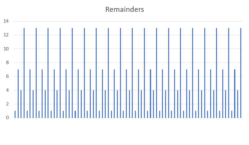
Figure 1. Plot of remainders shows inherent periodicity
Instead of a complex radio signal, we want to find the period of the remainders that, when plotted, looks like a signal (see Figure 1). Instead, we use a QFT, which allows us to find the period for integers large enough to break RSA and similar algorithms
In summary, the flowchart of Shor’s algorithm is as follows:
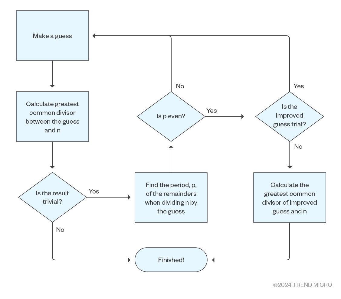
Figure 2. Shor’s algorithm flowchart
Background
We have glossed over many of the details with the promise of explaining them in succeeding sections. Let’s pick up these points and try to understand them better.
Getting from a guess to an actual factor
Why can we get factors of N from a guess? For some exponent of our guess, it should always be possible to find some multiplicand of N that nearly gets us to that value, and for the remainder, we can just add to that product. That is the reasoning behind the following equation:
$$ g ^{p} = m\quad\mathsf{x}\quad\mathsf{N}+ r$$
But what we want though is some expression that gives us two factors of N or, at least, something we can work with that gets us to that goal.
The first step is to make r = 1. With that, we have:
$$ g ^{p} = m\quad\mathsf{x}\quad\mathsf{N}+ 1$$
This can be rearranged by subtracting 1 from each side into:
$$ g ^{p} - 1 = m\quad\mathsf{x}\quad\mathsf{N}$$
If we squint a bit, the left-hand side is a recognizable polynomial, x2- 1, that we know how to factor into (x-1)(x+1). We can show that this is true by multiplying out (x+1)(x-1), from which we get x2+ x - x - 1 = x2- 1. We can do the same with our p, which becomes p/2 in the factors:
$$ (g ^{p\over2}+1)(g ^{p\over2}-1) = m\quad\mathsf{x}\quad N $$
The values of (g p⁄2 + 1) and (g p⁄2 - 1) are close to the factors that we are seeking, but as previously noted, when multiplied, they produce m × N. We need to find the greatest common divisor, which we previously glossed over. For this, we can use an ancient algorithm called Euclid’s algorithm.
Euclid’s algorithm
Since around 300 B.C., this algorithm has been used to efficiently find the greatest common divisor of two integers. Some improvements have occurred over the millennia and it now works as follows.
We start with a and b, which are the two integers we want to calculate the common divisor of and calculate the remainder, r, when we divide a by b. For example, if we try to divide 5 by 2, we get a remainder of 1 because the closest we can get by multiplying 2 by some integer is 4, which is 1 short of 5. At each step, if b is a nonzero, we compute the remainder, r, when dividing a by b. As a mathematical expression: a = m × b + r, for some m. Then the next step’s values are transferred by making the new a be the previous b and the new b be the previous r. For example, if we want to find the greatest common divisor of 50 and 15, we find how many times 15 goes into 50 and what the remainder is.
$$ a = 50, b = {15\to15} × 3 = {45\to50} = 45 + {5\to\mathsf{r}} = 5 $$
The next row’s a is the value in the previous row’s b, and the next row’s b is the value in the previous row’s r.
$$ a = 15, b = {5\to5} × 3 = {15\to15} = 15 + {0\to\mathsf{r}} = 0 $$
Again, the new a will be the previous b, and b will be the previous r:
$$ a = 5, r = {0\to } stop $$
The algorithm stops here, when b = 0 and we have found the greatest common divisor a = 5. We write gcd (50,15)=5.
Quantum Fourier transformation
We will pause for a moment and introduce something called a Fourier transform. A Fourier transform is a mathematical operation that takes an arbitrary signal in time (such as a sound wave) and produces a spectrum of frequencies for that signal. It has many applications in electronic systems that process signals, such as radio or sound.
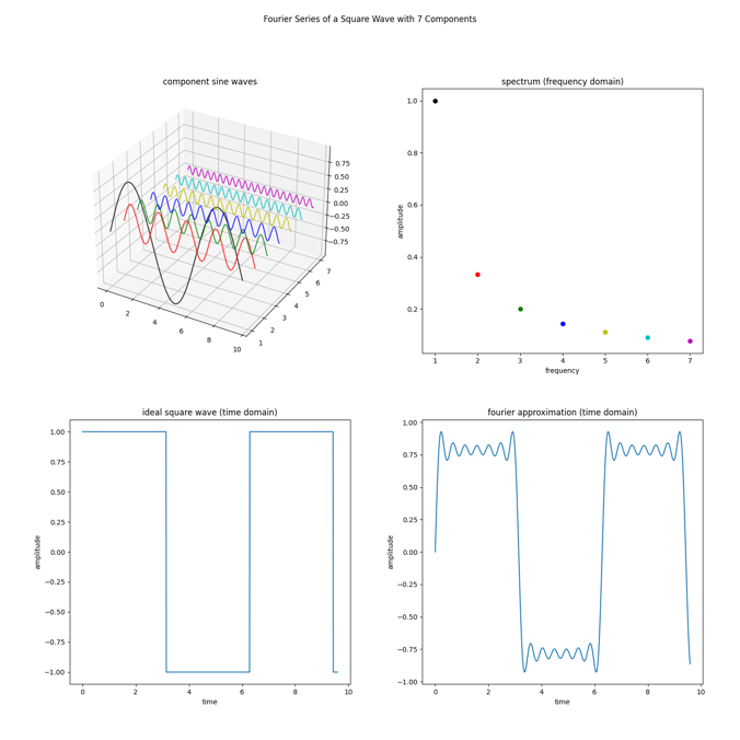
Figure 3. Fourier series of a square wave
The classic example of this is to take a square wave and decompose it into a series of sinusoidal waves that increase in frequency and reduce in amplitude. Figure 3 shows that by adding up sine waves, including the black, red, green, blue, olive , cyan, and magenta waves, we get something close to the square wave. If we add an infinite number of sine waves, we will eventually get a perfect square wave (dark blue). The square wave is in the time domain (left) and we can see a plot of which frequencies make it up in the frequency domain (right – these are the colored dots). Notice that for a square wave, it is all the odd harmonics added together that make up the spectrum. If the frequency of the square wave is f0, the primary wave will have the same frequency, f0. The harmonics will be: f1 is 3xf0, f2 is 5xf0, f3 is 7xf0,etc. This is the spectrum for a square wave signal. Other signals have other frequencies to compose them. Also note that the amplitudes of the frequencies diminish too, f0 is 1, f1 is 1/3, f2 is 1/5, f3 is 1/7. There is a nice pattern to this square wave.
Interestingly, the Fourier transform finds the periodicity of an arbitrary signal. That is exactly what we want in order to find our p and factor N.
Fourier transformations are not close to being fast enough for large cryptographic keys. The advantages of quantum computing include using the fact of superposition of all the possible powers of some number, x, and seeing this relationship between the different powers of x. Most of the mathematics is too involved and we will not be able to demonstrate this without going into much detail, but to put it very simplistically, we can instantly glean the periodicity, p, in the powers of x.
We start with a superposition of all possible powers with their respective remainders encoded onto qubits. The next step is to measure the superposition to get a random remainder in such a way that we are left with only the superpositions of all powers with the same remainder. Remember that these powers will be p apart regardless of which remainder we measured. Therefore, p is the period we see in the superposition of our output.
On a quantum computer, we need a little more than twice the qubits as the number of bits in N to factor it. This is because we need qubits to find the remainders and then use those in the quantum Fourier transformation. That is more qubits than any current gated quantum computer has, but not outside the realm of possibility. The catch is that we assume that we are using completely coherent qubits, but these are not feasible. Dealing with the problem of noise adds many factors to the number of qubits needed.
The quantum part of Shor’s algorithms, the part that calculates p, looks like this as a quantum circuit:
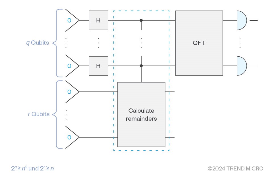
Figure 4. The part of Shor’s algorithm that calculates p
Symmetric cryptography and cryptographic hashes
Before concluding this article, it’s worth looking at hash algorithms and symmetric encryption. A hash algorithm uses multiple rounds of data “mixing” to form a fixed-length result. Hashes can be combined with cryptographic keys to form hash-based message authentication codes (HMAC) that can prove the integrity of a document. Symmetric encryption algorithms also mix plaintext data with a key to produce ciphertext, usually of the same length as the plaintext. We delve deep into symmetric algorithms in the first part of this four-part series.
Neither hashes nor symmetric encryption algorithms rely on the same class of problems that DHE (Diffie–Hellman key exchange), ECDHE (Elliptic-curve Diffie–Hellman), and RSA rely on. Consequently, a quantum computer running Shor’s algorithm will be of no use in attacking this type of cryptography. However, there is another quantum computing algorithm that does go some way toward attacking both hashes and symmetric encryption algorithms — Grover’s algorithm.
As we saw in the first article of this series, the best-known attack against the most common symmetric encryption algorithm, AES, is not much better than a brute-force trial of all potential keys in the keyspace. Once over half of the keyspace is tried, it’s more likely to have found the correct key, but it will take a very long time to accomplish. Grover’s algorithm uses the superposition of qubits to provide a faster search of the problem space.
For a function y = f(x), if the size of the key-space containing x is n, then our brute-force search to find x will take n/2 iterations on average. Grover’s algorithm can speed this up to about
For example, AES-128 has 128-bit keys, so, the size of its keyspace is 2128. A brute-force trial of 2127 keys should, on average, find us the right key, but that is a number of tries comparable to the number of atoms in the universe. This is why AES-128 is deemed secure today. With Grover’s algorithm, the number of keys to try is √2128 = 2128/2=264. This is still a large number. Consequently, even if a suitable quantum computer existed that could run Grover’s algorithm, we could achieve the same level of security as we have today simply by doubling our keyspace to 256 bits by using AES-256, which in the age of dedicated hardware support for AES and cheap storage, is an insignificant overhead.
Barring any unforeseen innovations, we can very easily make our symmetric key encryption and our hashing algorithms secure by just using larger keys. Our primary concern needs to focus on the key establishment protocols that rely on mathematical problems in the same class as integer factorization.
Conclusion
We have seen how cryptographic protocols that rely on integer factorization are susceptible to Shor’s algorithm that can find factors of very large integers given a gated quantum computer with enough qubits. This also holds for problems that are reducible to integer factorization, such as when they are in the same problem class, like elliptic curve cryptography. Shor’s algorithm is based on a foundational and well-explored algorithm that does Fourier transformations exponentially faster than any classical computer can.
By contrast, if we are worried about AES, then all we need to do is double the key size. This will result in finding the symmetric key using Grover’s algorithm being infeasible.
While we are close to building a quantum computer that has enough qubits to break these asymmetric key algorithms, in practice, their noisiness requires using large factors and more qubits than the theoretical minimum. Some estimates range from tens of thousands to tens of millions of qubits required and we are far from that.
Like it? Add this infographic to your site:
1. Click on the box below. 2. Press Ctrl+A to select all. 3. Press Ctrl+C to copy. 4. Paste the code into your page (Ctrl+V).
Image will appear the same size as you see above.
последний
- Fault Lines in the AI Ecosystem: TrendAI™ State of AI Security Report
- The Industrialization of Botnets: Automation and Scale as a New Threat Infrastructure
- From Holiday Snap to Custom Scam in 30 Minutes: How AI Turns Public Photos Into Targeted Attacks
- From LinkedIn to Tailored Attack in 30 Minutes: How AI Accelerates Target Profiling for Cybercrime
- Threat Attribution Framework: How TrendAI™ Applies Structure Over Speculation
 Fault Lines in the AI Ecosystem: TrendAI™ State of AI Security Report
 AI Security Starts Here: The Essentials for Every Organization
 The AI-fication of Cyberthreats: Trend Micro Security Predictions for 2026
 Stay Ahead of AI Threats: Secure LLM Applications With Trend Vision One